|
Design Guide
August 2003
|
 |
|
|
|
Electronic Filter Design Guide
|
|
DIGITIZING SIGNALS AND ALIASING
Analog to Digital Conversion (A/D)
Most physical (real world) signals are analog. Operating on these signals efficiently often requires the filtering, sampling and digitizing of the analog data using A/D converters. The converted digital data may then be manipulated mathematically. Many data-acquisition systems must also construct a representation of the original signal from the digital data stream.
Unfortunately, sampling often sacrifices accuracy for the sake of convenience. The digital version of a signal may not resemble the original in some important respects. A graphic example is the movie scene that apparently shows wagon wheels or helicopter blades turning backwards. This erroneous image, known as an "alias", occurs because a "motion picture" camera actually samples continuous action into a series of stills, and the frame rate (commonly 24 or 30 frames per second) is not fast enough or is nearly an exact multiple of the object's rotation speed.
According to Nyquist's Theorem, accurately representing an analog signal with samples requires that the original signal's highest frequency component be less than the Nyquist frequency, which is at least half the sampling frequency. To correct the image in the movie example, the frame rate would have to exceed twice the rotation speed of the wheel (or its spokes) or of the helicopter blades. No practical data-acquisition system can sample fast enough to catch all of a real signal's components. Frequencies above Nyquist appear as false low-frequency aliases. As an example, Figure 1 shows the result of sampling a 900 Hz signal at 1 kHz.
|

Figure 1
|
|
The process seems to indicate that the original signal was a 100 Hz sine wave, the difference between the actual input wave and sampling frequencies. Note that as the maximum signal frequency approaches the Nyquist frequency, the total number of samples needed to reconstruct the signal accurately approaches infinity.
Aliasing is a fundamental mathematical result of the sampling process. It occurs independent of any physical sampling-system capabilities. Downstream processing cannot reverse its effect. Only filtering out the alias high frequency components before sampling begins can prevent it.
When a signal undergoes A/D conversion, the amplitude of any frequency component above Nyquist should be no higher than the converter's least significant bit (LSB). Some sources insist on reducing the amplitude to below half of the LSB. For any full-scale undesirable signal component, then, attenuation should be at least 6 dB x n, where "n" is the number of bits in the A/D. For half of the LSB, attenuation would be 6 dB x (n + 1). A 12-bit A/D, then, demands attenuation of 72 dB or 78 dB.
In practice, noise-signal amplitudes rarely match the amplitudes of signal components of interest, so this attenuation calculation represents worst case.
IDEAL FILTER SHAPES (THEORETICAL)
Every electronic design project produces signals that require filtering, processing, or amplification, from simple gain to the most complex DSP. The following presentation attempts to "de-mystify" some of these signal-processing requirements. The concepts of ideal filters, commonly used filter transfer function characteristics and implementation techniques will assist the reader in determining their electronic filter and signal conditioning needs.
Real-world signals contain both wanted and unwanted information. Therefore, some kind of filtering technique must separate the two before processing and analysis can begin.
An ideal filter transmits frequencies in its pass-band, unattenuated and without phase shift, while not allowing any signal components in the stop-band to get through. All filters offer a pass-band, a stop-band and a cutoff frequency or corner frequency (fc) that defines the frequency boundary between the pass-band and the stop-band.
Figure 2 shows the four basic filter types: low-pass, high-pass, band-pass and band-reject (notch) filters. The differences among these filter types depend on the relationship between pass- and stop-bands.
|

Figure 2
|
|
Low-pass filters are by far the most common filter type, earning wide popularity in removing alias signals and for other aspects of data acquisition and signal conversion. For a low-pass filter, the pass-band extends from DC (0 Hz) to fc and the stop-band lies above fc .
In a high-pass filter, the pass-band lies above fc , while the stop-band resides below that point.
Combining high-pass and low-pass technologies permits constructing band-pass and band-reject filters. Band-pass filters transmit only those signal components within a band around a center frequency fo .An ideal band-pass filter would feature brick-wall transitions at fL and fH , rejecting all signal frequencies outside that range. Band-pass filter applications include situations that require extracting a specific tone, such as a test tone, from adjacent tones or broadband noise.
Band-reject (sometimes called band-stop or notch ) filters transmit all signals except those between fH and fL . These filters can remove a specific tone - such as a 50 or 60 Hz line frequency pickup - from other signals. A common application is medical instrumentation, where high-impedance sensors pick up line frequencies.
NON-IDEAL FILTERS (REAL WORLD)
Real-world signals contain both wanted and unwanted information. Therefore, some kind of filtering technique must separate the two before processing and analysis can begin. Real filters are far from ideal. They subject input signals to mathematical transfer functions with names like Butterworth, Bessel, constant delay and elliptic that only approximate ideal behavior. Instead of the sharply defined transition represented by ideal filters, real filters contain a transition region between the pass-band and the stop-band as shown in Figure 3.
|

Figure 3
|
|
In addition, the pass-band is not flat like the ideal filter, may contain attenuation ripple, and the attenuation in the stop-band may not be infinite. In order to simplify the analysis of various real world filter types, filter response curves are normalized. When selecting a filter, this normalized data allows the designer to compare the theoretical amplitude, phase and delay characteristics of each filter type.
Normalization
See Figure 4 below for the theoretical performance characteristics and normalized response curve of an 8-pole, 6-zero constant delay filter. The frequency axis on the response plot is scaled so that the corner or ripple frequency is always one Hertz instead of the actual intended corner or ripple frequency. This allows one normalized curve to represent any filter that would have the same response shape. To convert a normalized amplitude response curve to a curve representing a filter whose corner frequency is not at one Hertz, multiplying any number on the frequency axis by the intended corner or ripple frequency scales the frequency axis.
|

Figure 4 - Frequency Response
|
|
Amplitude Response
Amplitude Response is defined as the ratio of the output amplitude to the input amplitude versus frequency and is usually plotted on a log/log scale as shown in Figure 5. Note how the steepness of the transition band slope (roll-off) increases as the number of poles increase.
|

Figure 5 - 2, 4, 6, and 8 Pole Butterworth Lowpass
|
|
Phase Response
All non-ideal filters introduce a time delay between the filter input and output terminals. This delay can be represented as a phase shift if a sine wave is passed through the filter. The extent of phase shift depends on the filter's transfer function. For most filter shapes, the amount of phase shift changes with the input signal frequency. The normal way of representing this change in phase is through the concept of Group Delay, the derivative of the phase shift through the filter with respect to frequency.
| Group Delay (D) equation: |
D =
|
d
df
|
Group Delay
Group Delay is the phase slope on a linear phase vs. frequency plot. Figure 6 compares the group delay of some typical phase response curves.
|

Figure 6 - 8 Pole Lowpass, Group Delay Response
Butterworth, Bessel, Constant Delay, Elliptic
|
|
Thus a point on a normalized group delay curve that has a group delay of one (1.0) second would yield 1 millisecond Actual Delay for a filter with a 1KHz corner frequency.
| Actual Delay = |
|
Normalized Group Delay
|
|
Actual Corner Frequency (fc) in Hz |
| Actual Delay = |
|
1.0 sec
|
= 0.001 sec/Hz |
|
1000 Hz |
Analog Filter Specifications
Low-Pass and High-Pass
In order to define the limits of the filter pass-band in real circuits, most filter specifications define the corner frequency (fc), as the frequency where attenuation reaches -3 dB or for elliptic filters, the ripple frequency (fr), the point where the response curve last passes through the specified pass-band ripple. Filter specifications may also include a shape factor (sf) requirement, which describes how fast signals roll-off during transition. The sf represents the ratio between the cutoff/ripple frequency and where the filter achieves a desired attenuation level, say (-80 dB).
Figure 7 is an elliptic filter that attenuates to -80 dB at 1.56 fr, hence a shape factor of 1.56 to -80 dB. A high-pass filter with a 1.56 shape factor would achieve that same -80 dB of attenuation at fr/1.56 or 0.64 fr.
|
Filter Attenuation
|
|
(Theoretical) |
|
0.05 dB
|
|
1.00 fr
|
|
3.01 dB
|
|
1.05 fr
|
|
60.0 dB
|
|
1.45 fr
|
|
80.0 dB
|
|
1.56 fr
|
Also note that the elliptic transfer function attenuation floor is not infinite, but has notches and humps.
|

Figure 7
|
|
From the attenuation table above, this low-pass elliptic filter has a -3 dB frequency of 1.05 at fr, therefore the shape factor is calculated as follows:
Band-Pass and Band Reject Filters
Specific items of interest for Band-Pass filters are the Center Frequency (geometric mean) fo, the Filter Bandwidth, the Quality Factor (Q) and the shape factor.
Frequency fo represents the geometric mean of fH and fL. That is:
fo = (fH * fL ) 1/2
Bandwidth is defined as the difference between pass-band extremes:
Bandwidth = fH - fL
The Quality Factor (Q) of a band-pass filter represents the ratio of the center frequency fo to the -3 dB bandwidth
Following is an example of band-pass filter calculations:
|
Filter
Attenuation
|
|
fH/fo
|
|
fL/fo
|
|
-3dB
|
|
1.105
|
|
0.905
|
|
-80dB
|
|
2.414
|
|
0.414
|
fH(-3dB) - fL(-3dB) = 1.105 fo - 0.905 fo = 0.20 fo
fH(-80dB) - fL(-80dB) = 2.41 fo - 0.414 fo = 2.0 fo
| Therefore: Q(-3dB) = |
|
fo
|
= |
fo
|
= |
5 |
|
fH(-3dB) - fL(-3dB) |
0.2 fo |
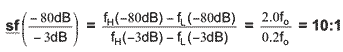
Figure 8 is a plot of a four pole-pair band-pass with a Butterworth transfer function and a Q of 5. For band-pass filters, the shape factor shows the ratio of the bandwidth at some attenuation level (say -80 dB) to the specified pass-band bandwidth (the bandwidth at -3 dB). Its shape factor at -80 dB is 10:1.
|

Figure 8
|
|
A Band-Reject filter's shape factor is the reciprocal of this number - that is, the ratio of the pass-band bandwidth to the corresponding bandwidth at the noted attenuatiopn level.
Filter Equations
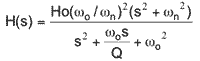
Filter transfer functions relate filter output to input through polynomials in the Laplace-transform complex variable "S" as shown in Equation 1. Using the "S" domain may seem confusing, but allows both the amplitude and time response of a filter to be expressed in a simple format. A two pole, two zero, low-pass filter can be expressed as:
Equation 1
where: Ho = dc gain
Q = peaking factor at the corner frequency
 o = 2 o = 2 fo = filter corner frequency fo = filter corner frequency
n = filter notch frequency
Filters may include both Poles and Zeros. A Pole is any frequency that makes the denominator of the mathematical transfer function go to zero. A Zero is a frequency that makes the transfer-function numerator go to zero. Second-order transfer functions may contain two poles and up to two zeros. To achieve steeper roll-off, higher-order real filters usually include cascades of second-order and first-order filter stages.
To produce the phase and frequency response, "S" in the above equation is replaced by j . Consider the second-order function that produces the amplitude versus frequency curve in Figure 9.
|

Figure 9

Figure 10
|
|
Linear-active filters can be made to closely match theoretical transfer functions. Cascading first and second-order filter sections easily produces three, four, five, six, seven, and eight-pole roll-off characteristics. Performance is as good as the operational amplifiers that they contain. With appropriate component selection, these filters contribute little broad-band-noise and can achieve distortion levels lower than -100 dB. Semiconductor switches permit corner-frequency programming without significant noise, distortion, or other undesirable effects. These filters are generally smaller than passive types for frequencies less than 100 kHz. Filter-section corner frequencies - and therefore the accuracy and shape of phase and amplitude curves - depend on amplifier characteristics, passive-component accuracy and stability.
ANALOG CIRCUIT DESIGN
Though there are several ways of constructing active filters, most applications use one of three topologies:
The Sallen-Key topology injects signal into the non-inverting input of the opamp, which is usually set for unity gain operation. This allows very accurate unity gain in the filter passband. Distortion can be a problem for the Sallen-Key design, as most opamps do not allow a large common mode signal swing without adding distortion to the signal. Only one opamp is needed to build a two-pole filter section.
The multiple feedback topology also uses one opamp for a two pole section, injecting signal into the inverting input of the opamp, usually with the non-inverting input grounded. This limits common mode input voltage swing and provides better distortion for larger signal swings. Gain set depends on resistor ratios, so pass-band gain is dependent on the accuracy of the resistors chosen. You can build high-pass filters in the multiple feedback form though the input impedance decreases to a very low value at higher frequencies. It is not possible to build multiple feedback filters with zeros. Multiple feedback topologies are not as versatile as other topologies.
For precision performance the state variable topology is the hardest to design but provides the most versatility. State variable designs require a minimum of three opamps and often are realized using four opamps to increase the versatility even further. Unlike the Sallen-Key and multiple feedback topologies, the state variable filter Q, fo and pass-band gain can all be independently set. This independence allows for higher precision filters because of the reduced component tolerance buildup. The state variable filter is the basis for most programmable filters.
An active filter's amplifiers contribute DC offset, although careful filter design can limit it to millivolt, and in many cases microvolt, levels. This error is usually stable with time and changes little with temperature. The amplifiers also add harmonic distortion to filter output. However, since active filters can achieve distortion levels less than -100 dB at frequencies up to 100 kHz and -110 dB at up to 20 kHz, they can easily pre-filter 16-bit (-96 dB) and 18-bit (-108 dB) A/D converters.
FILTER SELECTION
Transfer functions can be classified into one of two basic categories, Amplitude filters and Phase filters. Amplitude filters are designed for the best amplitude response for a given situation, for example zero ripple in the amplitude response pass-band. Phase filters are designed for desired phase response, such as linear phase with frequency throughout the filter amplitude pass-band.
Amplitude Filters
For many applications the design goal is to approximate ideal "brick wall" frequency response. Probably the most common amplitude filter transfer function is the Butterworth, which consists of an array of poles uniformly distributed on a left-half-plane unit circle, as in Figure 10A. This arrangement yields the maximally flat amplitude response in the pass-band (the first 2n - 1 derivatives of the frequency response are equal to zero, where n is the number of poles). Therefore, amplitude response rolls-off monotonically (uniform slope) as frequency increases in the stop-band.
The attenuation ratio "A()", of a Butterworth low-pass transfer function is given by:
where N = degree of the filter (number of poles).
Butterworth filters produce no pass-band ripple and provide theoretically infinite attenuation as frequency increases when compared to fc . The primary limitation is, Butterworth filters produce slower roll-off than some of the alternative transfer functions.
The attenuation ratio of a Chebychev transfer function (Figure 6C) is given by:

which generates a series of polynomials, where  is pass-band ripple and CN represents the nth order polynomial in the series. Table 1 shows the first five Chebychev polynomials. is pass-band ripple and CN represents the nth order polynomial in the series. Table 1 shows the first five Chebychev polynomials.
Chebychev Polynomials CN
| N |
|
CN |
|
1
|
|
|
|
2
|
|
22 - 1 |
|
3
|
|
43 - 3 |
|
4
|
|
84 - 82 + 1 |
|
5
|
|
165 - 203 + 5 |
Table 1
|
|
|
|
|
The Chebychev function provides faster roll-off in the transition band than a Butterworth filter would, but at the expense of some variation in the pass-band called ripple. Ripple denotes that the amplitude in the pass-band varies between 1 and (1 + 2), where is always less than 1. Pole frequencies are more spread out and the Q's of the sections are higher than the comparable section Q's of a Butterworth. Determining pole locations involves applying hyperbolic trigonometric functions to each pole of a Butterworth filter of the same order. Like the Butterworth, Chebychev stop-band roll-off is monotonic. It is important to note that many designers avoid Chebychev transfer functions in favor of Cauer elliptic alternatives because section Q's are higher for Chebychevs than with elliptic functions which provide faster roll-off in the transition-band.
Cauer elliptic transfer-function attenuation is given by:
where S = j , ZN is the nth order elliptic polynomial, and determines pass-band ripple attenuation at the cutoff frequency, = 1. Although an elliptic filter achieves faster roll-off than either Butterworth or Chebychev varieties, it introduces ripple in both the pass- and stop-bands. Also, elliptic filter roll-off is not monotonic, eventually reaching an attenuation limit, called the stop-band floor.
For elliptic filters, shape factor depends not on the -3 dB corner frequency (fc), but on ripple frequency (fr), the highest pass-band frequency on a low-pass filter or the lowest pass-band frequency on a high-pass filter where pass-band ripple occurs, as shown in Figure 11.
|

Figure 11
|
|
At the stop-band edge, a small frequency change produces a large change in attenuation. Another critical element in the shape of an elliptic filter is frequency fs, which denotes the first frequency at which the attenuation reaches the stop-band floor.
The pole configuration for this transfer function consists of a set of poles around an ellipse with pairs of zeros on the j axis, see Figure 10D. Pole frequencies are spread out over the pass-band. Section Q's are less than those in a comparable-order-and-ripple Chebychev. Desired pass-band ripple, stop-band floor and shape factor determines actual pole and zero locations in a particular filter. Figure 12 compares the amplitude response of eight-pole Butterworth, 0.1 dB ripple Chebychev, and 0.1 dB ripple, -84 dB stop-band floor Cauer-elliptic transfer functions. The curves are normalized to the -3 dB cutoff frequencies.
|

Figure 12
|
|
Generally, filters that produce faster roll-off in the transition-band exhibit poorer phase response and group delay characteristics (See Figure 6).
Phase Filters
For some filter applications it is desirable to preserve a transient waveform while removing higher frequency noise components from the signal. If each of the frequency components of the input waveform (from the Fourier series or the Fourier transform) is phase shifted an amount linearly proportional to frequency, then they remain in the correct time relationship and sum together to create, at the output, the original waveform that was present at the input of the filter, with the higher frequencies components having been removed by the filter. When a filter has phase delay that varies linearly with frequency it is called a Linear Phase filter. A linear phase filter has a constant group delay, at least through the pass-band. Amplitude filters provide relatively constant group delay only from 0 Hz to about the mid pass-band frequency range peak near fc.
As with amplitude filters, mathematicians have provided polynomial approximations of an ideal linear phase transfer function. The most common linear phase filter is based on Bessel (sometimes called Thompson) functions. Bessel filters provide very linear phase response and little delay distortion (constant group delay) in the pass-band. They show no overshoot in response to step input and roll-off monotonically in the stop-band. They also exhibit much slower attenuation in the transition-band than amplitude filters. Figure 13 presents amplitude and delay response curves for an 8-pole Bessel. Other types of phase filters include, constant-delay (a modified Bessel), equiripple phase, equiripple delay, and Gaussian transfer functions. They either have more pass-band amplitude roll-off for only a small improvement in phase linearity or only slightly less roll-off in the pass-band at the expense of degrading the phase linearity.
|

Figure 13
|
|
Compensated Filters
Some applications require filters offering the sharp roll-off characteristics of amplitude-type filters and the linearity of phase-type transfer functions. Two techniques, amplitude equalization and delay equalization, are available to achieve these ends. Both add complexity to filter design, and have theoretical and practical limits.
Amplitude equalization modifies the amplitude response of phase filters to produce a filter that is sometimes called a constant delay filter. Stop-band zeros on the j axis introduce attenuation notches in the stop-band, but contribute no phase or delay to the pass-band response. Figure 14 shows mirror-image right-half, left-half plane pass-band-zero pairs that modify amplitude response without additional phase or delay.
|
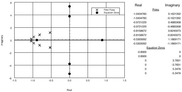
Figure 14
|
|
Improving the transition-band roll-off rate, however, does not come free. Adding zeros also introduces a small amount of step-input overshoot, and roll-off is no longer monotonic; that is, compensation introduces a stop-band floor. The j-axis zeros produce a "soft" or rounded roll-off near the cutoff frequency. These zeros become the dominant contributors to attenuation-curve shape, preventing further corner-frequency shape improvement.
This technique can achieve a factor-of-two improvement in Bessel roll-off to a -80 dB floor, comparable to Butterworth-filter performance. For comparison, Figure 15 shows the amplitude response of an 8-pole Bessel, an 8-pole, 6-zero constant delay, and a 8-pole Butterworth response.
|

Figure 15
|
|
Delay equalization employs additional all-pass (no attenuation) filter sections in cascade with standard filter sections to modify the phase linearity of amplitude filters. All-pass filters have left-half-plane poles and mirror image right-half-plane zeros. The pole and zero locations determine phase shift, though the added phase shift does not change the filters amplitude response. Adding phase shift at appropriate places in the pass-band allows, "straightening out" the phase curve of an amplitude filter. Each pole-zero pair of an all-pass filter increases phase shift from approximately 90º at fc to as much as 180º at 10 times fc. Therefore, adding equalizer sections increases total phase shift for the filter/equalizer network.
From a practical point-of-view, this technique allows filter and system designers an order-of-magnitude phase-linearity improvement over conventional amplitude transfer functions. Figure 16 illustrates the group delay of a 6-pole, 4-zero elliptic filter with and without a two-pole delay equalizer. The equalized plot is flatter over a larger portion of the pass-band at the expense of an increase in the amount of delay. The equalization process in this case increases total phase shift by as much as 360° at the cutoff frequency and by 720° at higher frequencies.
|

Figure 16
|
|
The number and location of poles and zeros in a delay equalizer depend on the pole configuration of the accompanying filter and the desired linearity improvement. Therefore, there are no "standard" solutions. Frequency Devices creates delay-equalization filters based on each situation and on each customer's specific requirements.
OUTPUT SIGNAL ERRORS
Besides inaccuracies of theoretical approximation, the most significant side effects of signal filtering are the following:
Settling time is not strictly an output signal error because it is mathematically related to the filter transfer function, but is usually deemed to be an undesirable filter side effect. All filters serve to delay the input signal by a certain minimum amount as well as increasing rise and fall time of any fast changing input signal. A general rule for settling time is that the more the filter approaches a "brick-wall" approximation, the longer it will take to settle. Therefore, an eight-pole filter will take longer to settle than a four-pole filter.
Step Response for amplitude type filters may exhibit substantial overshoot (ringing) when presented with a sudden change in voltage amplitude at the filter input. See Figure 17 for typical 8 pole transfer function step response curves.
|

Figure 17
|
|
DC-offset adds a voltage directly to an input signal to obtain the output value. Sophisticated systems may permit calibrating or compensating for this effect. When evaluating filters and A/D converters, designers must also consider DC-offset stability with time and temperature to ensure that compensation circuitry and procedures remain valid regardless of environmental conditions. For programmable filters, DC offset may vary with corner-frequency settings.
Noise (noise created by both passive and semiconductor devices) is present at the output of any filter. In most cases, later filter stages remove stop-band noise from earlier stages, but they leave noise in the pass-band unaffected. High-Q filter stages amplify noise near their corner frequencies. In an active filter, for example, the noise spectrum in the stop-band is usually flat and low level, resulting largely from the output amplifier. At the low-frequency end of the pass-band, the noise spectrum is also flat, but with a magnitude two to four times the level of the stop-band noise. Near the corner frequency, noise levels peak at magnitudes that depend on the filter's transfer function. Elliptic filters, which feature high-Q last stages, produce noise peaks near the corner frequency of three to five times the level of low-frequency pass-band noise.
The importance of noise will depend on the system bandwidth and the level of signals passing through the filter. In digitizing systems, aliasing folds a frequency spectrum around each harmonic of the sampling frequency, and because these effects are additive, achieving the best data accuracy requires reducing broad-band-noise as much as possible.
Distortion, harmonics of the input signal's frequency components result from non-linearity in the filter circuit. These harmonics become inputs to the A/D converter, which digitizes them with the rest of the signal. As with broad-band-noise, each low-pass filter stage removes stop-band distortion components that the previous stage generates. Distortion levels vary with input-signal frequency, amplitude, transfer function, and corner frequency.
Total Harmonic Distortion (THD) is a specification often used as a single number representation of the distortion present in the output of an active circuit. It is the RMS sum of the individual harmonic distortions (i.e. 2nd, 3rd, --- etc.) that are created by the non-linearities of the active and passive components in the circuit when it is driven by a pure sinusoidal input at a given amplitude and frequency.
Harmonic distortion measurement requires a very low distortion sinusoidal input to the circuit, the removal of the fundamental frequency component from the output and the measurement of the amplitude of the remaining harmonics, which are typically 60 to 140 dB below that of the fundamental.
Spectrum analyzers and FFT instruments can measure individual harmonic components and can be used to calculate the THD. For active filters, the THD is usually specified in dBc (dB relative to the amplitude of the fundamental frequency component) and at a specific frequency and amplitude (ex. 10Vp-p @ 1.0kHz).
An RMS voltmeter can be used to measure the THD if, the fundamental frequency component can be removed by a notch filter to a level that is at least an order of magnitude below the largest harmonic component. However, that measurement will also include any noise that is within the bandwidth of the meter and is commonly referred to as the THD + NOISE or THD + N.
At lower frequencies, amplifiers have sufficient loop gain to reduce distortion to acceptable levels. For input frequencies near fc, the filter removes second and higher order harmonics. Above the corner frequency, filter attenuation reduces the primary signal, which also reduces the distortion. However, if` the signal frequencies are well below the corner frequency and the signal has distortion, then that distortion will also reside in the filter's pass-band. Distortion components will affect the accuracy of the analog-to-digital signal conversion.
SELECTING THE RIGHT ANALOG FILTER
Choosing the correct filter shape for a particular application requires defining properties of the incoming signal that the filter must remove, as well as the properties that it must retain. In most situations, there is some overlap between these two areas, demanding a degree of compromise.
Time Domain Waveform Preservation
Filters for such applications feature linear phase response in the pass-band, and must not introduce ringing or overshoot. To preserve the signal waveform while removing undesired components, the filter must also pass many harmonics of the incoming signal's base frequency. "Noise" components that the filter removes must be at substantially higher frequencies than these necessary harmonics. Phase-derived filters, such as Bessel or constant-delay (equiripple-phase) and their amplitude-compensated derivatives, work best in these cases.
High Selectivity in the Frequency Domain
Situations where removal of undesired components is the overriding concern and some distortion in the time domain of the signal's shape is of less importance generally require sharper roll-off filters with Butterworth or elliptic transfer functions. Spectrum analysis, for example, involves only the amplitude of each frequency component of the input signal. Most voice and data transmission also requires integrity only of amplitudes, as do many forms of modal analysis, which determines resonant frequencies of structures and objects.
Compromise Filters
Although linear-phase filters preserve critical information, many applications also require rapid transition-band roll-off. A balance between these mutually exclusive requirements can often be achieved by phase-derived types and amplitude-compensated versions of phase filters. Applications for this approach include determining the direction of an object or signal source by analyzing the waveform from one or more receivers.
|
|
|
|
|
|
|